Supporting effective municipal government through education, training, advocacy, and legal services since 1941.

Tech Insights: Utilizing NHMA’s Wage Data Part 3
The information contained in this article is not intended as legal advice and may no longer be accurate due to changes in the law. Consult NHMA's legal services or your municipal attorney.
I will be continuing to use the Wage Data downloaded from NHMA’s website (see the May/June and July/August 2026 issues) to show how you may wish to utilize the data. For a quick recap, I have downloaded wage data, resized the columns, froze the top title row and the columns A and B, and formatted the minimum and maximum columns to be in comma format.
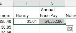
A review of the data shows there are three different salary types – Hourly, Salary, and Stipend. I want to convert all non-stipend wage data to the same format – either hourly or annual base pay. Because there is also a salary range, I will take the average of the minimum and maximum at the same time. Although most users will want the data converted to one format or the other, I will add two columns, one for hourly and another for annual base pay. To do this quickly, I will highlight columns F and G which are currently Notes and Last Updated (Date). Right click anywhere in the highlighted area and choose insert. Excel will insert two columns already formatted the same as the column directly to the left of where you inserted the new columns. This means the new column F and G are both already formatted the same as column E, Maximum, in the comma format. I will add the titles of Hourly and Annual Base Pay to the new columns. Annual Base Pay does not fit within the width of the column. I could resize the column to fit the title, but then the column is wider than I need it for any of the data that will appear. Instead, I will tell the text to wrap which will also automatically resize the row height. To do this, click in the title cell, G1. Now go to the Home tab and in the Alignment section click on the (wrap) icon. Not only does the text wrap, but the row height automatically adjusted to allow both lines of the wrapped text.
Next, in the Hourly columns, I want to convert the average of all salary items to hourly, average the hourly, and show the stipend amounts as zero. Because I know the data in column C, Salary Type, are one of three options, I can use the IFS function in Excel. The IFS function checks the conditions of a cell or function and returns the first true condition met. In this case, I will go to cell F2, the first row of data under the new Hourly column. In that cell I will type the following function. If your fulltime hours are different than 40 hours a week or 2080 a year, replace the 2080 with your annual number of hours such as 1950 for a 37.5 work week.
=IFS(C2="Salary", AVERAGE(D2:E2)/2080, C2="Hourly", AVERAGE(D2:E2), C2="Stipend", 0)
If you prefer, you can always use the Insert Function option to enter in formulas / functions. In either case, the function tells us to average the minimum and maximum of the salary positions and bring that down to an hourly rate, or average the hourly rate, or place a zero in the cell if it is a stipend. By defining each of those three choices, that leaves the possibility of a blank field if data in column C has accidentally been altered.
The function for column G, Annual Base Pay, is very similar and is as follows.
=IFS(C2="Salary", AVERAGE(D2:E2),C2="Hourly", AVERAGE(D2:E2)*2080, C2="Stipend",0)
To save my typing and possibly showing off my not so exemplary typing skills, I copied the formula from F1 into G1. BUT, in order to preserve the cell references, I cannot just copy the cell and paste into another. I click in cell F2 so the function appears in the function box above the cells. I then highlight the entire function and either right click, copy or CTL C. Both options copy the function to the computer’s clipboard. Finally, I click in cell G2, the first data row of the Annual Base Pay column and either right click, paste or CTL V to paste. This method preserves the cell references without Excel trying to be helpful by adjusting the columns over one. Finally, I remove the “/2080” from the salary option and add “*2080” to the hourly option.
To quickly bring those formulas down every row, I highlight both cells F2 and G2. In the lower right corner of the highlighted section there is a black square. Double clicking that square will automatically copy the formulas down to every cell where there is date in the cell directly to the left, column E (Maximum) in this case.